on
Blog Post 5
Week 5 - The Air War
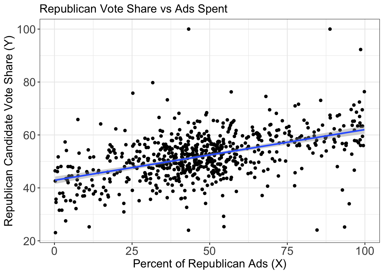
For this week’s blog, I will be delving into the concept of ad buys and how this may impact congressional races. To do this, we will be trying to build a model where we look at what impact the number of ad buys has on the eventual turnout of the race. As you will see below, we are looking at ads from the years 2006 to 2018. While we have the number of Democratic ad buys and the number of Republican ad buys in any given district, the independent variable of interest will actually be the percentage of Republican or Democratic ad buys out of all of the total ad buys in that district. In this case, I decided to use Republican vote share as the outcome, so I will be seeing what impact the percentage of Republican ad buys has on the turnout for Republicans in the race.
As the below model shows, we are able to see some trends where an increase in the percentage of Republican ad buys leads to a small increase in the number of Republican vote percentage in that district. This makes sense because having a greater share of the ads in a district shoudl help you in the election. However, as you can also see below, we have a rather low R-Squared value close to 0.23, so it is possible that a lot of this variance in is not actually being explained by the variance in ad buys. A large part of this, as I will get into, is because of the severe limitations of this dataset.
##
## Call:
## lm(formula = adVoteShare$repAdPercent ~ adVoteShare$RepVotesMajorPercent)
##
## Residuals:
## Min 1Q Median 3Q Max
## -62.427 -12.435 -0.428 11.319 78.426
##
## Coefficients:
## Estimate Std. Error t value Pr(>|t|)
## (Intercept) -15.51708 4.49545 -3.452 0.000592 ***
## adVoteShare$RepVotesMajorPercent 1.21176 0.08524 14.216 < 2e-16 ***
## ---
## Signif. codes: 0 '***' 0.001 '**' 0.01 '*' 0.05 '.' 0.1 ' ' 1
##
## Residual standard error: 19.99 on 669 degrees of freedom
## (21 observations deleted due to missingness)
## Multiple R-squared: 0.232, Adjusted R-squared: 0.2308
## F-statistic: 202.1 on 1 and 669 DF, p-value: < 2.2e-16
To furhter visualize this, I also have a plot of Ad percentage vs vote percentage here.
Next, I will get into the limitations of the dataset. Below, I have plotted the total number of Democratic and Republican ads by congressional district in the year 2018 in the two maps below. As you can see, a large number of the districts don’t have any color to them because they are showing up as NA. This is due to two things. The first is that in large numbers of districts which likely aren’t competitive, candidates may not be running ads and we also may not have access to the data on if they are. While this makes sense that these district won’t have ads, this also means that the years of 2006 to 2018 give us access to less data and it is harder to make a model. Furthermore, I believe that some of the NAs should not actually show up as none but it is due to error in the dataset.
Next, I will get into some pitfalls. The first pitfall I would like to explain is the lack of available data from 2022. Even if we had this data, it would be very hard to update my ongoing national model because as I already explained it did not create a good model. However, we also simply don’t have access to 2022 ad data, so we will not be updating the 2022 predictions for this week because of that.
With this in mind, I would like to pivot to another pitfall of the work we have been doing with ad buys, which is Gross Rating Points or GRPs and can help us think more about why ad buys themselves might not be a very predictive vatiable.
Gross Rating Points (GRP) is a measure of how many people are watching television programming when an ad is aired. This is really important because in arguably this is more meaningful than fundraising or ad spending is. Even if assume that ad spending is effective in persuading some voters, ad spending on its own is only impactful if people actually see the ads. We calculate this score by thinking about the percent of the ad’s media market that will see the ad. For example, in the article, Huber et al say that a GRP of 50 would mean half of the households in a media market saw a given ad. With this data, we can do things like see how a candidate’s advantage in spending (spending peaks) might correspond with higher GRPs. With this in mind, I would think that in order to approximate advertising effects at the national level like a Huber type study or even at a district level, we would want to use the lessons from the readings and consider not just the amount of ads being aired or bought but also the amount of viewership of the ads through things like the GRP. Especially for district level races where a lot of the races might not have large numbers of ads being aired, looking at the viewership of ads might allow us to tell if advertising truly mattered. For example, if we saw a correlation between a candidate’s peak in support and the amount of advertising being spent, but then also saw that the ads had very low viewership or had low GRPS, we may want to question whether or not the ads were casuing the peak in support. Maybe more ads are bought when outside factors are causing high levels of support and the campaign has more money. While it would be difficult for us to hone this conclusion down entirely, having access to information like GRPs and potentially seeing that some ads actually weren’t even being viewed at high levels might allow us to conclude that the advertising was not the important factor at play.